Nearly five years ago, Zachary Stevens and co (PloS Biology, 2015) extrapolated a trend in genomic data generation for ten years, predicting an exciting and terrifying future of exabyte-scale genomic datasets in the early 2020s. The genomics community had experienced 3x year-over-year data growth that indicated no sign of slowing down, and analyzing the largest datasets with existing tools was becoming infeasible. Geneticists processing these datasets were spending less time doing science, and more time implementing and running even basic analyses.

The Hail project began in the year 2015, and was tasked with building open-source, scalable tools to enable geneticists to interrogate the largest genomic datasets. Hail has since evolved from a command-line VCF-processing tool to a versatile Python library used for data manipulation and analysis, with a wide array of functionality specifically for genomics.
Core Features
Genomic Dataframes
Modern data science in nearly every domain is powered by dataframe libraries. Pandas, R’s Tidyverse, SAS, SQL engines, and many other tools are designed to process data consisting of observations (rows) of heterogeneous fields (columns). However, these tools cannot easily and efficiently represent genomic data.
Analysis-ready genomic datasets have rows (sites in the genome that vary across individuals), columns (sequenced individual identifiers), and a third dimension, the several fields comprising the probabilistic measurement of an individual’s genotype at a specific site. Hail represents this type of dataset in a first-class way with a core piece of the Hail library, the MatrixTable.
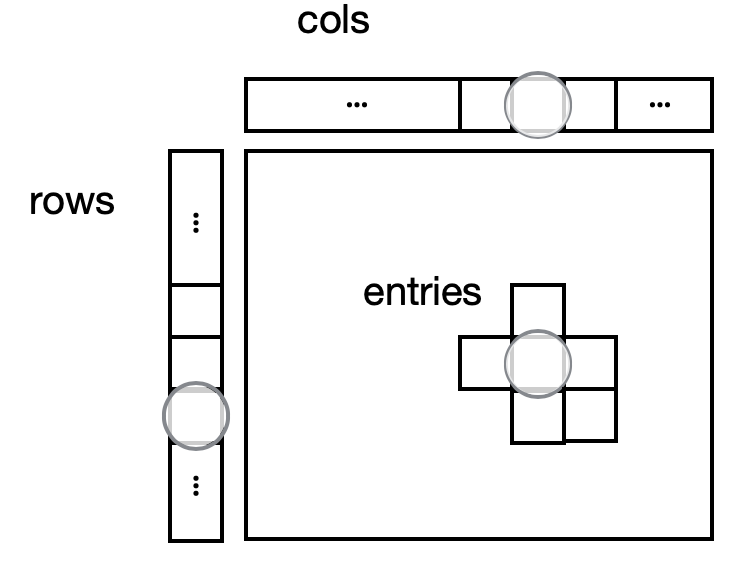
MatrixTable: The rows table stores row fields that have one value per row (variant) like locus, alleles, and variant annotations. The cols table stores column fields that have one value per column (sample), like the sample ID and phenotype information. The entries are a two-dimensional structured matrix that can contain genotype fields like GT, DP, GQ, AD, and PL. Finally, global fields have only one value. Adapted from the Hail cheatsheet: https://hail.is/docs/0.2/cheatsheets.htmlTip: see names and types of fields at any point with mt.describe()
Simplified Analysis
Hail functionality is built around the MatrixTable interface. This is the core unifying interface for import, export, exploration, and statistical analysis.
Many input formats, one interface
In genomics, there are many file input formats and data representations. Hail unifies the various genomic data formats by importing them to the same data structures, Hail Tables and MatrixTables. Examples of Hail-compatible input formats include the variant call file (.vcf), tab-separated values (.tsv), Oxford genotype (.bgen, .gen), PLINK, gene transfer format (.gtf), browsable extensible data format (.bed), as well as other textual representations.
>>> mt = hl.import_vcf(‘data/example.vcf.bgz’,
                       reference_genome='GRCh38')

>>> mt = hl.import_gen('data/example.gen',
                       sample_file = 'data/example.sample')

>>> mt = hl.import_plink(bed='data/test.bed',
                         bim='data/test.bim',
                         fam='data/test.fam',
reference_genome='GRCh38')1) Filter, group, and aggregate
Most exploratory data analysis is built on standard dataframe operations: filtering, grouping, and aggregation.
>>> mt = mt.filter_rows(mt.variant_qc.AF[1] < 0.05)>>> mt = mt.annotate_rows(mean_allele_depth=hl.agg.mean(mt.AD)) >>> ti_tv_ratio = mt.aggregate_rows(
hl.agg.count_where(hl.is_transition(mt.alleles[0], mt.alleles[1])) /
hl.agg.count_where(hl.is_transversion(mt.alleles[0], mt.alleles[1])))2) Annotation.
Easy annotation in a single line for databases such as the variant effect predictor (VEP) or the genome aggregation database (gnomAD).
>>> mt = hl.vep(dataset)>>> gnomad='gs://gnomad-public/release/3.0/ht/genomes/gnomad.genomes.r3.0.sites.ht'
>>> gnomad_ht = hl.read_table(gnomad)
>>> mt = mt.annotate_rows(gnomad=gnomad_ht[mt.locus, mt.alleles])
3) Visualization. Hail includes a plotting library built on bokeh that makes it easy to visualize fields of Hail tables and matrix tables.
>>> p = hl.plot.scatter(x=mt.sample_qc.dp_stats.mean,
                        y=mt.sample_qc.call_rate,
                        xlabel='Mean DP',
                        ylabel='Call Rate',
                        size=8)
>>> show(p)
>>> p = hl.plot.manhattan(gwas.p_value)
>>> show(p)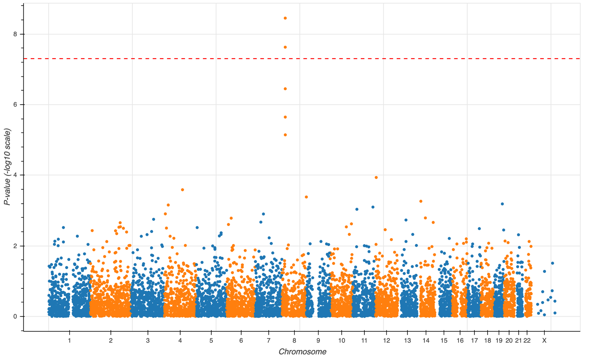
4) Statistical analysis toolkit
Hail features a suite of functionality for standard statistical genetics models.
>>> eigenvalues, scores, _ = hl.hwe_normalized_pca(mt.GT)
>>> mt = mt.annotate_cols(sample_pcs = scores[mt.s])>>> gwas = hl.linear_regression_rows(
y=mt.phenotype,
x=mt.GT.n_alt_alleles(),
covariates=[1.0,
mt.is_female,
mt.sample_pcs.scores[0],
mt.sample_pcs.scores[1],
mt.sample_pcs.scores[2]])Effortless Scalability
Hail can be used to interrogate biobank-scale genomic data.
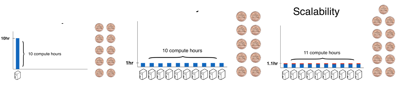
Scalability. It’s not feasible to process tens or hundreds of thousands of whole genomes on a single computer. Hail has a backend that automatically and efficiently scales to leverage a compute cluster, such as one deployed on-demand on the cloud, so that users can worry about the contents of their pipelines, rather than how to parallelize them. This means that it’s possible to have the same interactive analysis experience, whether the Jupyter notebook is running on a laptop or backed by 5,000 CPUs on a cloud cluster.
By using more computers, Hail can run large computations in a short amount of wall time, or how long users need to wait for results. Scalability does not come for free, though: even though the wall time decreases when using large clusters, the CPU time (wall clock time multiplied by average number of compute resources, and a proxy for cost) will slightly increase. A perfectly scalable system could run on a huge number of computers without inflating CPU time, making all queries interactive at no additional cost.
Perfect scalability is not feasible, but Hail comes acceptably close -- Hail achieves a ~300x speedup in runtime at ~2x cost.
Efficiency is the total amount of CPU time a tool uses, which translates into how much an analysis costs. Less efficient tools take longer to run, and therefore cost more. More efficient tools can utilize computer hardware better, taking less total time and therefore costing less.
The Hail team is invested in improving both scalability and efficiency. We believe that this is necessary to keep pace with growing genomic datasets.
How do I get started with Hail?
Hail can be run on multiple computational platforms:
Laptop. It’s easy to run Hail on a single machine, like a laptop, for small data. It’s easy to use a laptop to build and test analyses before running them on a full dataset on the cloud.
Cloud. Hail installations come bundled with a tool (hailctl dataproc ) that can be used to manage Hail clusters running on Google Dataproc on Google Cloud Platform (GCP). Hail can also run on Google Cloud with Terra, as well as on Amazon Web Services (AWS) and Microsoft Azure using community-built tooling.
Head to the Installation page to get started.
More functions, and how-to guides are available in the Hail documentation.
What has Hail produced (so far)?
Hail has seen robust adoption in academia and industry by enabling those without the expertise in parallel computing to flexibly, efficiently, and interactively analyze large genomic datasets. In the past few years, Hail has been the analytical engine behind dozens of studies, ranging from large-scale projects such as the Genome Aggregation Database (gnomAD), the Neale lab’s UK Biobank rapid-GWAS, and most recently, the driving force in the Pan-ancestry genetic analysis of the UK Biobank (Pan-UKBB).
To date, more than 50 publications have cited Hail in published research, and the Hail Python package has been downloaded from the Python Package Index more than 140,000 times.